Each year, the matchups for professional football leagues such as the CFL are decided deterministically based on a rotating schedule. With the matchups decided, these leagues are then faced with a combinatorial optimization problem: They have to schedule the games across a number of weeks such that they meet several constraints and optimize for secondary goals such as broadcast deals. This is a variation of the Nurse Scheduling Problem, and it's NP-hard. Some leagues approach this problem using "hundreds of computers in a secure room". In the future, they might be able to replace those computers with a quantum annealer.

What is Quantum Annealing?

Quantum annealing (QA) is a metaheuristic for finding the global minimum of a given objective function over a given set of candidate solutions (candidate states), by a process using quantum fluctuations (in other words, a meta-procedure for finding a procedure that finds an absolute minimum size/length/cost/distance from within a possibly very large, but nonetheless finite set of possible solutions using quantum fluctuation-based computation instead of classical computation).

That's the Wikipedia definition. In simpler terms, if we define a function that maps a candidate solution to a score, quantum annealing can help us find candidate solutions that minimize that score. In some ways it's like training a machine learning model, during which you aim to find a set of parameters that minimizes some loss function when evaluated against your training data.

Quadratic Unconstrained Binary Optimization (QUBO)

The technique we'll be exploring is called "quadratic unconstrained binary optimization". QUBO uses a cost or "energy" function that looks like this:

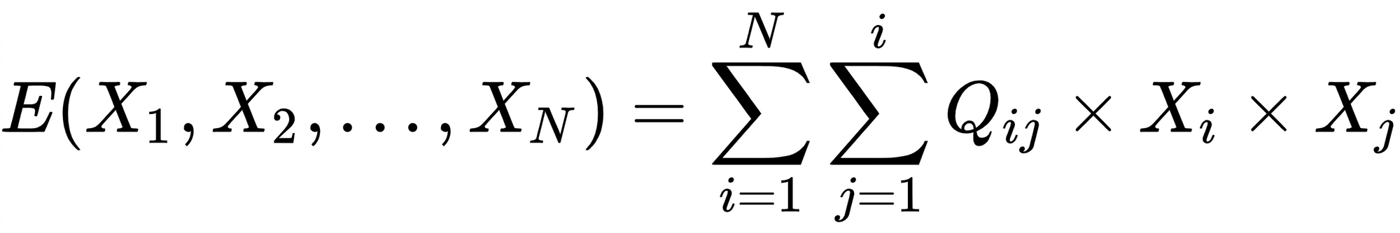
This function maps N binary parameters to an energy which is the sum of each element in the Q matrix for which X_i and X_j are 1. To schedule N football games across M weeks, we'll need N * M binary variables and a square matrix with N*M rows and columns. Our constraints can then be defined by filling out the Q matrix. For example, to encourage the annealer to schedule as many games as possible rather than leave the schedule empty, we can set the diagonal of the matrix to some negative number so that the energy is lowered by all variables that are set to 1.

Building the Q Matrix

We're going to schedule a football season with 4 constraints:

• Each game must be played.
• No game should be played twice.
• No teams should play twice in one week.
• The games should be spread evenly across all weeks.

The definitions will be written in Python. The focus of this post isn't really the code, but if you'd like to follow along using AWS Braket, you can my Jupyter notebook here.

To begin, we need to organize our matchups and create the empty Q matrix:

games = ['A@B', 'B@C', 'C@D', 'A@D']
n_games = len(games)
n_weeks = 2


def get_index(game_index, week_index):
    return game_index * n_weeks + week_index


Q = defaultdict(int)
e_offset = 0

We've decided on 4 games and decided that we're going to spread them across 2 weeks. That means we'll have 8 variables and Q will be a 8x8 matrix, where get_index(0, 0) gives us the index of the variable corresponding to game 0, week 0. e_offset will be used to adjust the overall energy of the solutions such that an ideal solution has exactly 0 energy.

Each game must be played.

As mentioned above, we can encourage the annealer to schedule every game by giving the games a negative cost:

cost = -5.2
for game in range(n_games):
    for week in range(n_weeks):
        idx = get_index(game, week)
        Q[idx, idx] += cost
e_offset -= cost * n_games

While not strictly, necessary, we adjust e_offset here to compensate so the resulting energy of an ideal solution is 0.

No game should be played twice.

cost = 3.5
for game in range(n_games):
    for week1 in range(n_weeks):
        idx1 = get_index(game, week1)
        for week2 in range(week1 + 1, n_weeks):
            idx2 = get_index(game, week2)
            Q[idx1, idx2] += 2 * cost

If a game is scheduled for multiple weeks, a penalty is applied.

No teams should play twice in one week.

games_by_team = {}
for i in range(n_games):
    for team in games[i].split('@'):
        team_games = games_by_team.get(team, [])
        team_games.append(i)
        games_by_team[team] = team_games

cost = 3.5
for game1 in range(n_games):
    for team in games[game1].split('@'):
        for game2 in games_by_team[team]:
            if game2 > game1:
                for week in range(n_weeks):
                    idx1 = get_index(game1, week)
                    idx2 = get_index(game2, week)
                    Q[idx2, idx1] += cost

This is very similar to the previous constraint except that it applies a penalty when a team plays twice within the same week.

The games should be spread evenly across all weeks.

cost = 0.3
for game in range(n_games):
    for week in range(n_weeks):
        idx = get_index(game, week)
        Q[idx, idx] -= cost * (n_games / n_weeks - 1)
for week in range(n_weeks):
    for game1 in range(n_games):
        idx1 = get_index(game1, week)
        for game2 in range(game1 + 1, n_games):
            idx2 = get_index(game2, week)
            Q[idx1, idx2] += cost
e_offset += 0.5 * n_games * cost * (n_games / n_weeks - 1)

This applies a penalty based on the number of games in each week. Each week contributes 0.3*(x-1)*x to the overall energy where x is the number of games in the week. Because energy increases exponentially based on the number of games in each week, the best solutions will have evenly spread games. The incentive to schedule games must be increased as well to balance out this penalty (Otherwise the weeks will be capped at a certain maximum number of games.).

Simulated Annealing

We can quickly test our Q matrix using simulated annealing before running on quantum hardware:

from dimod import BinaryQuadraticModel, SimulatedAnnealingSampler

bqm = BinaryQuadraticModel.from_qubo(Q, offset=e_offset)
sampler = SimulatedAnnealingSampler()
results = sampler.sample(bqm)


def show_results(results):
    smpl = results.first.sample
    energy = results.first.energy
    size = n_games * n_weeks
    print('Size: {}'.format(size))
    print('Energy: {:.6f}'.format(energy))

    for week in range(n_weeks):
        week_games = []
        for game in range(n_games):
            if smpl[get_index(game, week)] == 1:
                week_games.append(games[game])
        print('Week {}: {}'.format(week + 1, ', '.join(week_games)))


show_results(results)

The results might look something like this:

Size: 8
Energy: 0.000000
Week 1: A@B, C@D
Week 2: B@C, A@D

That's a perfectly valid schedule given our input and constraints. The energy of this solution is zero, which means it's what's known as a Ground State.

Quantum Annealing

The simulated annealing results were great, but quantum annealers are the future. Under the right circumstances, a D-Wave can be 10⁸ times faster than simulated annealing. We'll be testing this on a D-Wave 2000Q hosted by AWS Braket:

from braket.ocean_plugin import BraketDWaveSampler
from dwave.system.composites import EmbeddingComposite

s3_folder = ('MYBUCKET', 'simulation-output')
sampler = BraketDWaveSampler(s3_folder, 'arn:aws:braket:::device/qpu/d-wave/DW_2000Q_6')
sampler = EmbeddingComposite(sampler)
results = sampler.sample(bqm, num_reads=1000)
show_results(results)

Size: 8
Energy: 0.000000
Week 1: A@B, C@D
Week 2: B@C, A@D

Amazing! But... not really. Anyone could have put together that schedule without any real thought. Let's try generating an alternative schedule for the entire 2019 CFL season, which consists of 9 teams playing a total of 81 games over 21 weeks.

---------------------------------------------------------------------------
ValueError                                Traceback (most recent call last)
<ipython-input-4-1f1d7d8783d5> in <module>
      4 sampler = BraketDWaveSampler(s3_folder, 'arn:aws:braket:::device/qpu/d-wave/DW_2000Q_6')
      5 sampler = EmbeddingComposite(sampler)
----> 6 results = sampler.sample(bqm, num_reads=1000)
      7 show_results(results)

~/anaconda3/envs/Braket/lib/python3.7/site-packages/dwave/system/composites/embedding.py in sample(self, bqm, chain_strength, chain_break_method, chain_break_fraction, embedding_parameters, return_embedding, warnings, **parameters)
    244 
    245         if bqm and not embedding:
--> 246             raise ValueError("no embedding found")
    247 
    248         bqm_embedded = embed_bqm(bqm, embedding, target_adjacency,

ValueError: no embedding found

😱 Okay, let's take a break from QUBO to talk about the D-Wave 2000Q's hardware limitations.

Qubits and Chimera Graphs

A qubit is the quantum equivalent of a classical bit. It's the most basic unit of quantum information and the capabilities of quantum machines are largely dictated by how many qubits they have. The D-Wave 2000Q has 2048 qubits. This is a lot compared to the qubit counts of universal quantum computers such as the IonQ and Rigetti Aspen-8. However, the D-Wave is not a universal quantum computer. It is a device that specializes specifically in annealing, so the number of qubits that the device has only tells part of the story. The qubits on the D-Wave 2000Q have connectivity that forms the shape of a "chimera graph". The chimera graph consists of 64 cells, each with 8 qubits connected like so:

The 64 chimera cells in a D-Wave 2000Q are connected in a grid like so:

When we use QUBO, each variable requires a qubit. Furthermore, each variable must be physically connected to every other variable for which Q_ij is non-zero. If we scale our scheduling problem down a bit to 15 games over 5 weeks, we can visualize what our connected qubits have to look like:

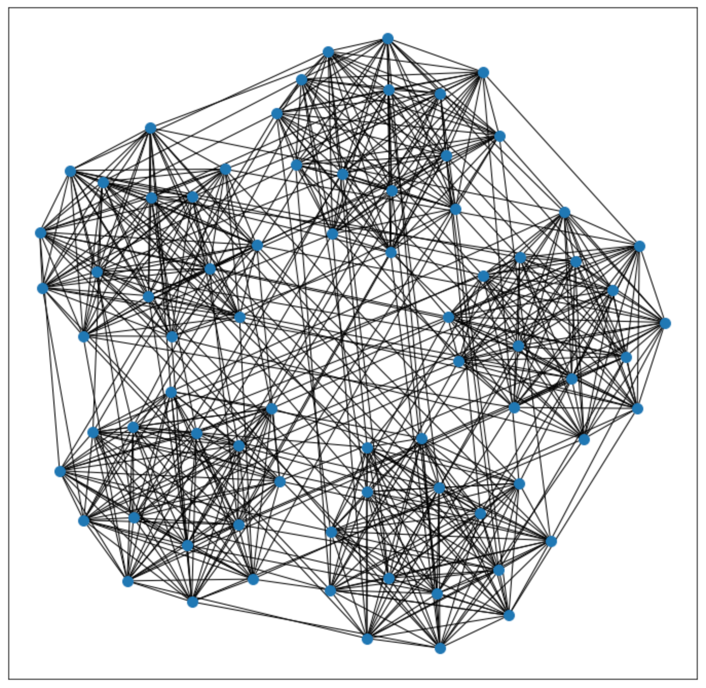
We have a total of 75 variables, which each need their own qubit. That should be no problem since the device has 2048 qubits. However, each of our variables is connected to every other variable for the same week and every other variable for the same game in different weeks. In other words, each qubit needs to be connected to 18 other qubits. We could say that this graph has a "degree" of 18. As you can see in the chimera graphs above, the D-Wave's qubits just don't have that kind of connectivity.

Embedding

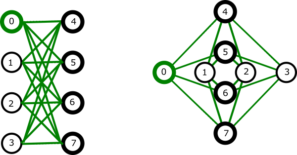
In order to perform annealing with higher degree graphs, we have to embed our graph onto the D-Wave's chimera graph. Embedding in this context can be thought of as a way to use multiple qubits for a variable in order to increase that variable's connectivity. If we scale our problem down even further to 8 games over 2 weeks, our unembedded graph looks like this:

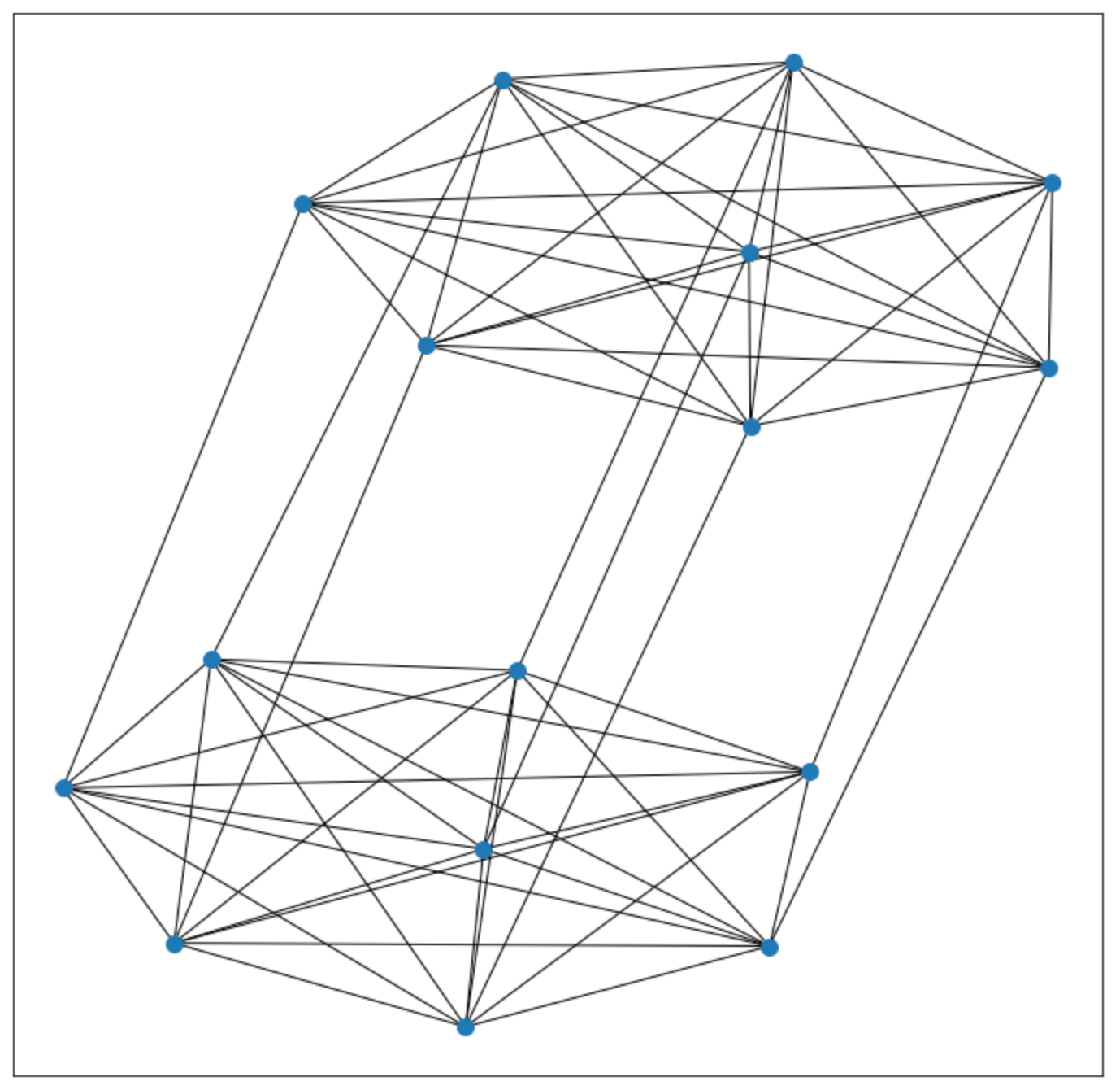
The degree of this graph is 8, which is still higher than the maximum degree of the D-Wave's chimera graph. To work around that, we can embed it like so:

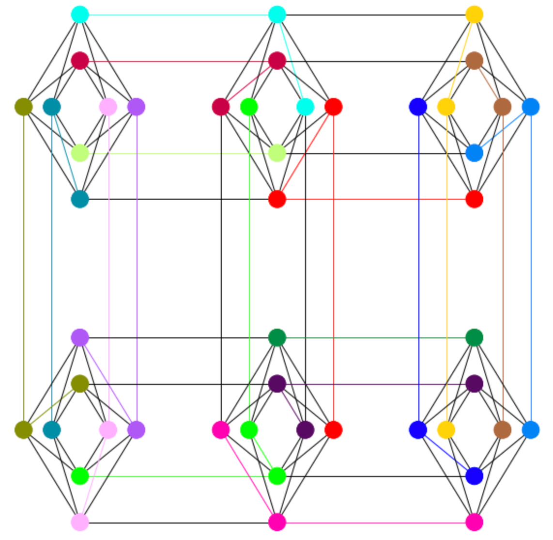
This is the same graph, but each variable is now represented by multiple qubits, allowing for higher connectivity. For example, all of the red qubits might be used to encode the variable for game 1, week 1. We can see in the graph that all of the red qubits are connected to each other, and together connect to at least 8 other qubits.

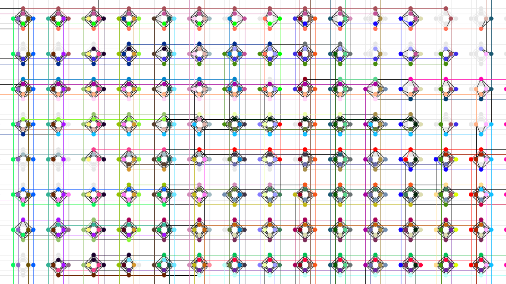
Now that we understand the physical constraints of our quantum annealing, let's take a look at the embedding for the 15 games over 5 weeks case:

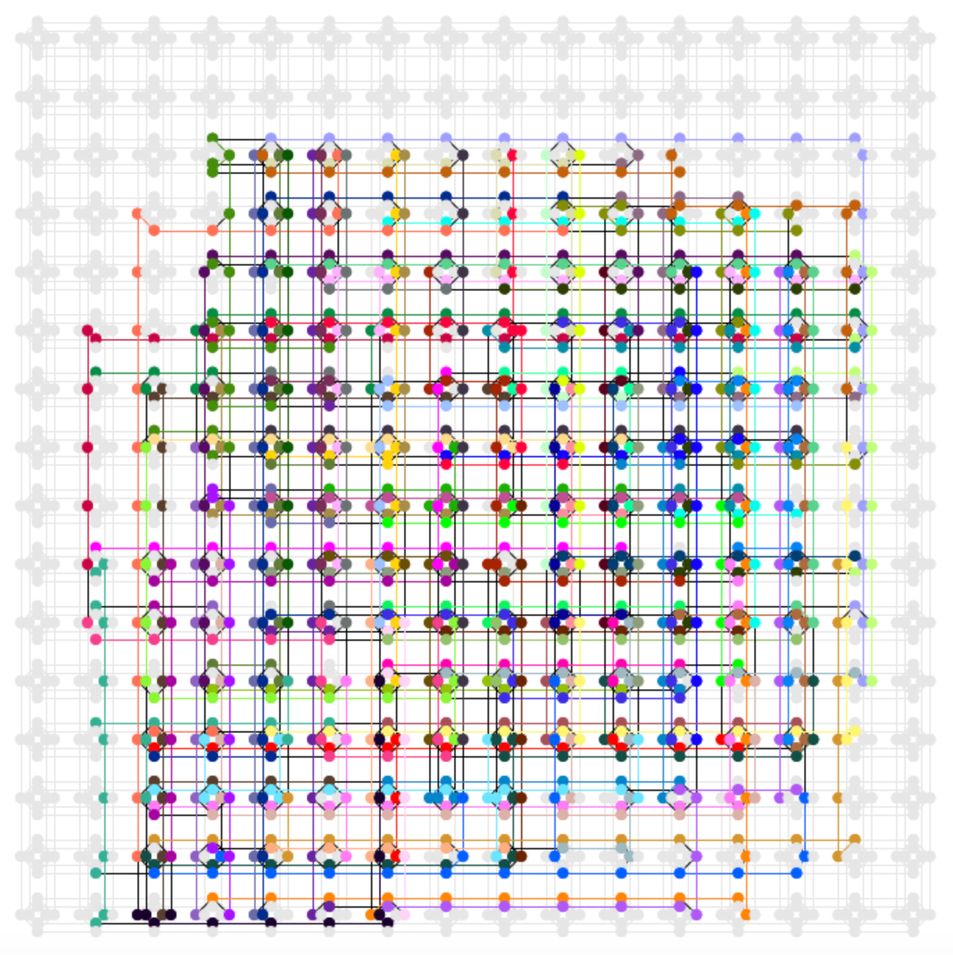
We can see now that despite only having 75 variables, we require most of the D-Wave's available qubits. Scheduling the entire season at once with this method and these constraints is a no-go for now.

Simulated vs Quantum Ground States

We've come this far, so let's go ahead and see what happens when we try to schedule 15 games over 5 weeks. First we'll try simulated annealing again:

Size: 75
Energy: -0.000000
Week 1: OTT@CGY, BC@EDM, HAM@MTL
Week 2: HAM@TOR, EDM@WPG, CGY@SSK
Week 3: MTL@HAM, BC@CGY, TOR@SSK
Week 4: SSK@HAM, WPG@OTT, BC@TOR
Week 5: MTL@EDM, WPG@BC, SSK@OTT

It's not as zippy as it was when we tried it with only 4 games, but simulated annealing does find a ground state for us. Perfect!

Now let's try quantum annealing on the D-Wave again:

Size: 75
Energy: 32.100000
Week 1: OTT@CGY, EDM@WPG, MTL@HAM
Week 2: WPG@OTT
Week 3: BC@CGY, TOR@SSK, HAM@MTL
Week 4: BC@EDM
Week 5: BC@TOR

With an energy of 32.1, this is clearly not a ground state. The quantum annealing failed to schedule all of the games. For this type of problem and scale, it's apparent that quantum annealing struggles more with finding ground states.

Conclusion

By tweaking our Q matrix and using more advanced techniques such as reverse annealing, we could almost certainly achieve a higher probability to reach ground states via quantum annealing. But regardless, due to the hardware limitations on problems with large numbers of variables, professional football leagues are probably going to be using their secure rooms with hundreds of computers (a.k.a. "AWS EC2") for a while.